Thin sections of grainflow with pinstripes

Locale: Page, Arizona, USA
GPS coordinates: 36.93515, -111.48979 (WGS84)

Two thin sections were prepared of grainflows with pinstripes in a sample of cross-stratified Jurassic sandstone from a road cut near Page, Arizona (likely Navajo Sandstone, but possibly Page Sandstone). The sections are perpendicular to the grainflow plane, and orthogonal to each other: One is dip-parallel, and the other is strike-parallel. This web page presents the context of the samples and then some analysis.

Zoomable, full resolution, downloadable versions of many of the images can be found at links in the Supplementary section at the bottom of this page.

Pinstripe

Pinstripe

Fig 1. Left, a photo of the cut surface of the sandstone that was subsequently impregnated with blue-dyed epoxy and thin sectioned, at the right. The two images are scaled so that the two pinstripes (marked by labels at the right margin) are aligned. The cut surface is not flat; the sandstone is so lightly-cemented that grains have fallen loose.

Figure 2, below, shows the sample (figure 4) in situ, located beneath the key, in the wall of a road cut (in figure 3, at yellow arrow) along highway 89, a few hundred meters west of Glen Canyon Dam (see GPS info at top of this page), near Page, Arizona.

There is at least a vertical meter of grainflow cross-strata above and below the sample. The base of the cross-strata is not exposed, but the exposed cross-strata are linear, with no sign of the flared wind ripple deposits commonly found near the base of a dune.

Fig 2. The top of the sampled rock is at the tip of car key.

Fig 3. The sample was from grainflow cross-strata in Navajo Sandstone. It was deposited on a dune slipface, at least a meter above the dune toe.

Figure 4 shows the sample on a rock saw table, with one cut already made. Two thin sections will be obtained, orthogonal to each other and the pinstripes, indicated by yellow and red lines. The black-marker arrow on the sample indicates dip direction. One thin section is parallel to dip, the other parallel to strike (perpendicular to dip). The thin sections cross the three pinstripes labelled p1, p2, and p3 in figures 4 and 5.

Fig 4. The thin sections come from the vertical planes in the locations indicated by the red and yellow bars. One is parallel to the palaeo-slipface dip, the other is parallel to strike; both are perpendicular to the slipface. The labels p1, p2, and p3 locate the three pinstripes that appear in the thin sections. The black arrow on the sample is in the direction of down dip.

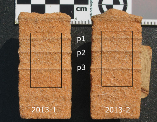
Fig 5. The black lines mark where the thin sections were obtained, approximately 5 mm beneath that surface. The labels p1, p2, and p3 correspond to the pinstripes in figure 4.

The sandstone held up well enough to the rock saw cuts, yielding the blocks shown in figure 5. The thin sections came from about 7 mm beneath the surface of the blocks in figure 5, below the positions marked by thin black lines.

The thin sections were prepared by National Petrographics in Texas, USA. Blue epoxy impregnation was requested, to hold the grains together, make grain boundaries obvious, and to eliminate voids that could be contaminated by particles generated during processing. It appears this was only partially successful; figure 7 shows grain-shaped 'ghosts' that suggest grains pulled away during cutting or grinding, and the returned off-cuts (eg., right-most object in figure 6) had numerous pits. Viewed through a microscope, the pits appear to be either created by grains pulled from the epoxy (leaving a bowl-shaped pit), or voids not filled by epoxy (deeper and irregular); the latter could perhaps have been avoided or reduced by vacuum impregnation (not available at National Petrographics).

Fig 6. The thin section slides are positioned such that the three pinstripes, labelled p1, p2, and p3, are aligned, and with the off-cut (at the right). The pits in the off-cut are caused by grains that pulled out during processing, and probably by voids in the epoxy impregnation (not performed under vacuum).

Fig 7. Yellow arrows mark outlines left probably by grains that pulled out of the epoxy during processing. The white rim may be due to refraction and/or grain coating left behind.

Figure 8, below, is a stereo pair of a part of the surface of an offcut, showing pits left by pulled grains and unfilled voids.

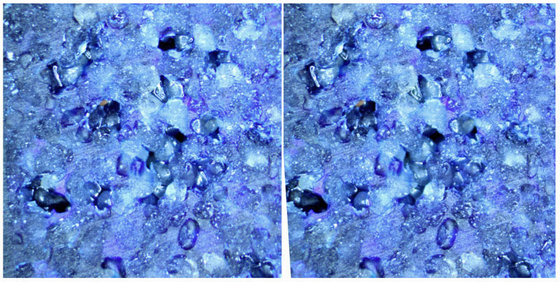
Fig 8. Stereo pair of the surface of an offcut, with pits due to pulled out grains and incomplete epoxy impregnation. Can be viewed by crossing one's eyes until the images overlap.

The large, irregular voids in the offcuts could be unfilled voids that were in the sandstone, but would grainflow have voids that size, and that would survive the approximately 30% compaction that this sandstone has undergone (changing the slipface dip angle from about 34° to about 26°)? This suggests the large voids in the offcuts are due to grains lost in processing.

The thin sections do not have as many clear areas as one might expect from the offcut void density, so perhaps additional blue epoxy was applied after cutting, before (or after) grinding and affixing to the slide.

The sections were stained for calcite (Alizarin Red S).

Figure 9, below, compares a view of the coarse saw-cut sandstone surface with the thin section that was obtained from about 7 mm below that surface (after impregnation with blue-dyed epoxy). Given that there are few or no cut or broken grains in the saw-cut surface, apparently the saw blade tended to knock loose grains rather than cut them, leaving the surface we see. After sawing, the sandstone surface was suspended in water, face down, to encourage any loose grains or 'rock dust' to drop away.

As discussed above, large voids in both views are likely due to lost grains.

These are cropped views at 66% of full resolution. Full resolution images are available from links referenced in the Supplementary section at the bottom of this page.

Fig 9. Left, a photo of the sandstone surface prior to epoxy impregnation. Right, the thin section produced from the area about 5 mm beneath the photographed surface. The two images are scaled to align. This is sample 2013-1, which is strike-parallel. Only a portion of each image is shown; full images are linked in Supplementary Data.

ImageJ was used to perform particle analysis, which involves classifying areas of the thin section image as either background or particle ('threshold analysis'), establishing particle boundaries ('watershed'), manually reviewing and improving upon that result, and then finally generating particle statistics (location, dimensions, etc). See Appendix for details.

Likely there will someday be artificial intelligent tools to isolate grains in an image, but meanwhile, I just used what is included in standard ImageJ and spent only a few hours with Photoshop fixing up the grain boundaries it identified (see the Supplementary section for the post-processed binary images).

I filled in some 'ghosts' in voids where it was obvious that a grain had pulled out, but I was not thorough about it; also I made an only modest effort to fix up the isolation of small particles within pinstripes. Thus the results are only a suggestion of the true distributions. The resulting data for each thin section are available in spreadsheets from the Supplementary section.

A standard thin section is 30μm thick, and thus these thin sections capture the intersection of the sandstone grains with a plane 30μm thick. Even if all the grains were an identical diameter, the resulting thin section would have a range of apparent grain diameters, due to variation in where the plane passed through a particular grain. In sandstone with grains of varying sizes, a large grain cut off-center might appear in the thin section similar to a smaller grain cut at its widest point. Here that effect is ignored; grain diameters are taken as being as they appear in the thin section.

Below is some analysis, using R to produce the charts. Particle diameter is calculated as the geometric mean of the minimum and maximum Feret's diameter, produced by ImageJ's particle analysis routine (consult ImageJ documentation for more info).

Fig 10, below. A trimmed area of the thin section of sample 2013-1 (strike parallel) is shown on the right, bordered to the left and below by charts showing the distribution of grain sizes along each dimension. The points are fitted by the R 'loess' function, with a smoothing parameter (span=0.1) and an approximate 95% confidence band. The curves at the line ends are edge artifacts.

The shape of the blue line is strongly dependent upon the smoothing parameter selected, and thus is only a suggestion of the distribution.

The inter-pinstripe grain population beneath the bottom pinstripe has less larger grains than the other three inter-pinstripe populations.

There is a layer, about 2mm thick, of medium-size grains immediately above the lowest pinstripe.

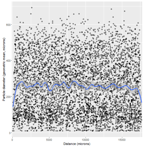
Laterally, parallel to strike, the distribution of grain sizes seems uniform.

Below, figure 11, are the distributions along the dimension perpendicular to the slipface for the two thin sections, side by side.

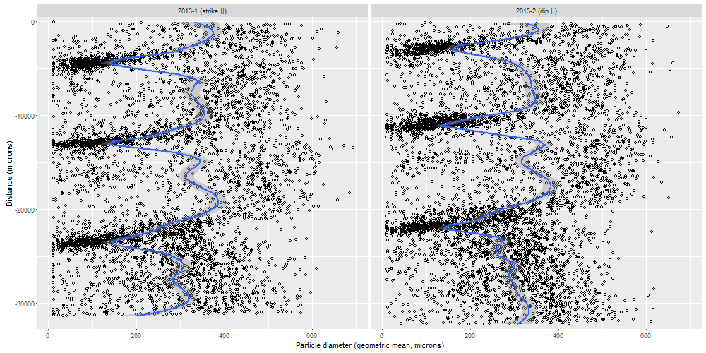
Fig 11. Grain size distributions along the dimension perpendicular to the slipface for the two thin sections, side by side. The points are fitted by the R 'loess' function, with a smoothing parameter (span=0.1) and an approximate 95% confidence band. The curves at the line ends are edge artifacts.

Below, figure 12, are the distributions along the dimension parallel to the slipface for the two thin sections, side by side.

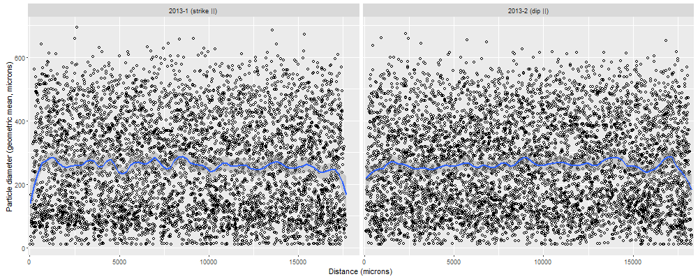
Fig 12. Grain size distributions along the dimension perpendicular to the slipface for the two thin sections, side by side. The points are fitted by the R 'loess' function, with a smoothing parameter (span=0.1) and an approximate 95% confidence band. The curves at the line ends are edge artifacts.

Below, figure 13, are histograms of overall grain size distribution for the two thin sections, with curves fitted, showing a bimodal distribution.

Recall that this is based upon less-than-perfect semi-automatic identification of grain boundaries by image analysis of the thin sections, and ignores that the apparent grain diameter in thin section would be less than true if the cutting plane happened to pass through a grain away from its widest point.

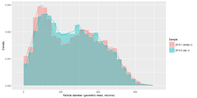
Fig 13. Overall grain size distribution for the two thin sections, with curves fitted

Software & versions

ImageJ 1.50e
Photoshop CS5 12.0.4
RStudio 0.99.491
R 3.2.3, with ggplot2 2.0.0

Related

Appendix

Methods, software, and steps used to produce images and perform particle analysis.

ImageJ

These are the ImageJ steps to obtain particle analysis results from the thin section images:

R

These are the R commands used to process the results files (produced by ImageJ->AnalyseParticles) and create charts:

library("ggplot2")

g1<-read.table('particles_2013-1.txt')
g1$Sample<-'2013-1 (strike ||)'
g1$sampleNum<-1

g2<-read.table('particles_2013-2.txt')
g2$Sample<-'2013-2 (dip ||)'
g2$sampleNum<-2

g<-rbind(g1,g2)
g$FeretAve<-sqrt(g$Feret * g$MinFeret)
g$yBin<-findInterval(g$YM,seq(0,max(g$YM),l=50))
g$fBin<-findInterval(g$FeretAve,seq(0, 700, l=11))

ggplot(g, aes(x=-YM, y=FeretAve))+geom_point(shape=1)+geom_smooth(method="loess", span=.1)+
  coord_flip()+scale_x_continuous(name="Distance (microns)", expand=c(0,500))+
  scale_y_continuous(name="Particle diameter (geometric mean, microns)")+facet_wrap(~Sample)

ggplot(g, aes(x=XM, y=FeretAve))+geom_point(shape=1)+geom_smooth(method="loess", span=.1)+
  scale_x_continuous(name="Distance (microns)", expand=c(0,100))+
  scale_y_continuous(name="Particle diameter (geometric mean, microns)")+facet_wrap(~Sample)

ggplot(g, aes(FeretAve, fill=Sample)) +
  geom_histogram(alpha = 0.4,aes(y=..density..),position='identity',binwidth=25) +
  geom_line(stat='density',aes(colour=Sample),alpha = .5, adjust=.5,size=1) +
  xlab("Particle diameter (geometric mean, microns)")+ylab("Density")

Supplementary

Full resolution, downloadable images, and results of particle analysis:

2013-1 (strike parallel)

Image: sandstone surface (7 MB) (Google Photos; use controls to zoom to full resolution with full screen)
Image: thin section, full resolution (35 MB) (Gigapan; use controls to zoom to full resolution with full screen)
Image: thin section, quarter resolution (4 MB) (used to generate particle mask)
Image: particle mask (<1 MB), scale is 8.80343 μm/pixel
Spreadsheet (tab-separated text): particle analysis results (<1 MB)

2013-2 (dip parallel)

Image: sandstone surface (7 MB)
Image: thin section, full resolution (35 MB) (Gigapan)
Image: thin section, quarter resolution (4 MB) (used to generate particle mask)
Image: particle mask (<1 MB), scale is 8.83392 μm/pixel
Spreadsheet (tab-separated text): particle analysis results (<1 MB)